The first year of my MSc has finally come to pass, which is great, because I can finally start thinking about my research project - which is what I’m really excited about. I’m going to be creating a library in Julia to implement the Fast Multipole Method in 3D, that takes advantage of the parallelisation offered by modern hardware. This algorithm has a reputation for being complex, with few expositionary resources for learning about it at a postgraduate/senior undergraduate level, so I’m also going to make a dedicated website visualising the algorithm in different physical contexts, giving me the chance to play around with JavaScript and D3.js.
In this post I was planning on giving a cursory motivation for why this is an interesting problem in computer science and applied maths, as it’s a relatively straightforward problem to understand. I’m going to be using some mathematical notation, but nothing really beyond what’s covered in a standard A Level maths course. However instead of going through the Fast Multipole Method, I’ll go through the slightly easier to interpret Tree Code, which gives an impression of how these fast methods could work at all.
Modelling Pairwise Interactions
The $N$ body problem is probably the best starting point. It’s a suprisingly common physical situation, where you want to evaluate a function $N$ times at $N$ different points. For example, when modelling the gravitational interaction between particles of matter, in order to find the potential from the other $N-1$ particles at a given particle for all $N$ particles, a direct calculation would be of $O(N^2)$ complexity.
More rigorously, we can state the problem as follows. Given a set of $X \subset \mathbb{R}^d$ of $N$ target points, and $Y \subset \mathbb{R}^d$ source points, some ‘kernel’ function to be evaluated linking these two sets of points together $G(x, y)$, and perhaps a set of weights at each source point $f(y)$, our evaluation boils down to the following sum at each target point,
$u(x) = \Sigma_{y \in Y} G(x, y)f(y)$
For example in simulating particle interactions, $X$ and $Y$ would be the locations of each particle, and if we were evaluating gravitational potential $G(x, y) = \frac{1}{\left | x- y \right | }$, and $f(y)$ the relative weight of each particle. This is well known from Physics as a Coulomb potential, used in both modelling electrostatics as well as classical gravity.
For simplicity, we’re going to stick to a 2D domain ($\mathbb{R}^2$), where the system we are considering models this Coloumb interactions between particles (fig A).
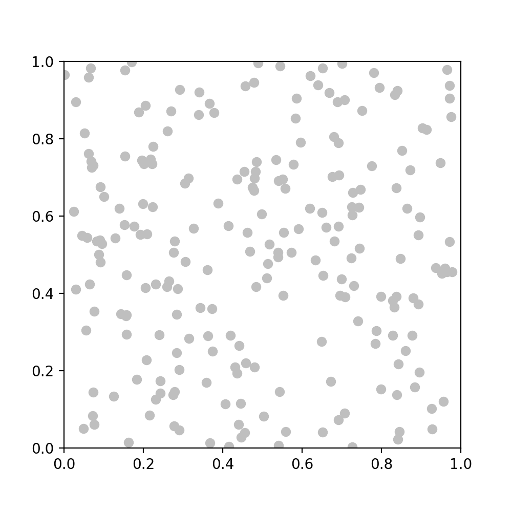 A. Quasi-Random Uniform Distribution
Our goal is to compute all pairwise interactions. Considering two square subregions of the domain, marked $A$ and $B$, if $A$ and $B$ are disjoint, in the sense that there’s strictly no overlap between them (fig B),
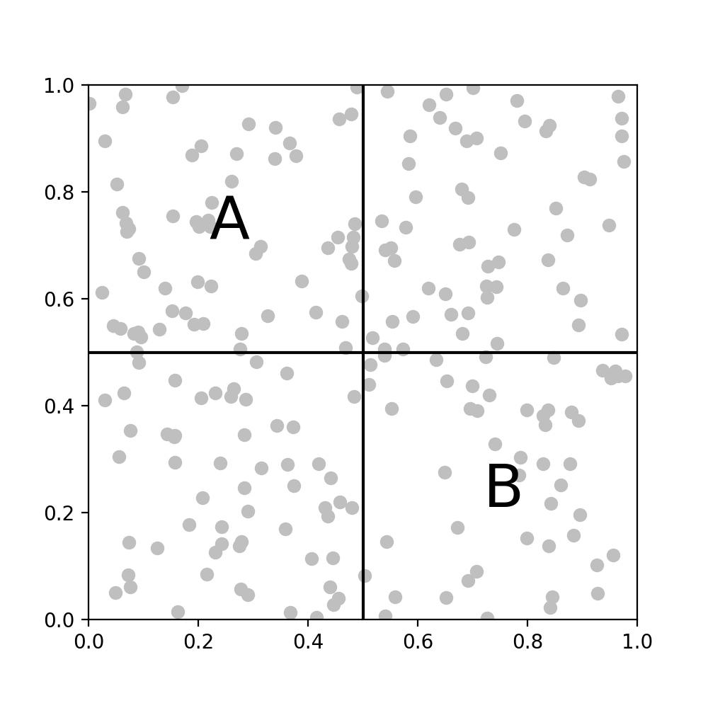 B. Disjoint $A$ and $B$
then we can make the following approximation. Consider $A$ and $B$ as an Astronomer modelling the gravitational interaction between two galaxies. If both are ‘well separated’, in the sense that we can treat the distributed mass of all the matter in the galaxy as a single point, then our $O(N^2)$ evaluation of the potential between these two galaxies goes to a much simpler $O(N)$ calculation (fig C).
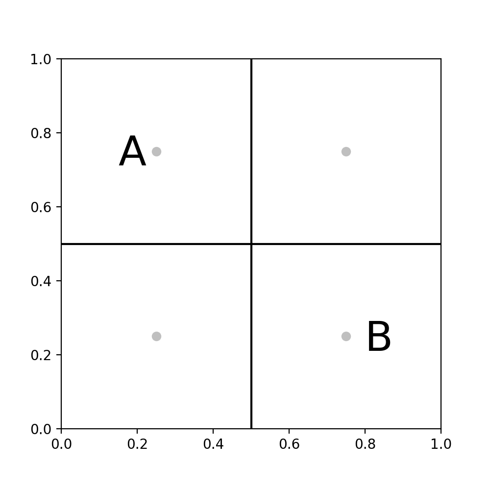 C. $A$ and $B$ treated as points
This only partly solves the problem, as we now have a way to model the interaction between $A$ and $B$, but we need a way to repeat similar approximations accross all the points in the domain. We can get around this by repeatedly partitioning the domain into a quadtree structure until, the number of points in each leaf box is less than some $O(1)$ constant (fig D).
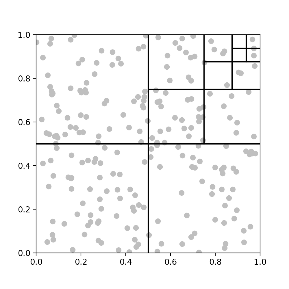 D. Repeated partitioning of domain, illustrated on one quadrant
The whole ‘quadtree’ has $O(\log N)$ levels and at each level $l$ (starting at 0), there are $4^l$ squares, giving $O(N/4^l)$ points in each box. Denoting the top level, with no partitioning, as level 0, the algorithm starts at level 2. Let $B$’s near field be it’s direct neighbours, and the far field be the complement of the near field. For a box $A$ in the far field, we can use the summarisation technique described above. In the first step (fig E) both $A$ and $B$ contain $O(N/4^2)$ points. The algorithms consists of the summarisation operation, which will have to be completed $4^2$ times, and the $O(1)$ evaluation of the potential. This results in an $O(N)$ complexity, and we’ve succesfully computed all of the interactions in $B$’s far field. To find the interactions from its near field, we have to recurse down to the next level on the quadtree, level 4. A bunch of interactions have already been taken care of on the previous level. We repeat the procedure from the previous level, finding the far-field interactions on $B$. Finally, we reach the leaf level where have $O(N)$ nodes left, which are bounded by some small constant. We can then just sum these up by direct computation in $O(N)$ steps. We see that the direct calculation has been reduced from $O(N^2)$ complexity, and is now bounded by $O(N \log N)$ as there are in $O(\log N)$ levels.
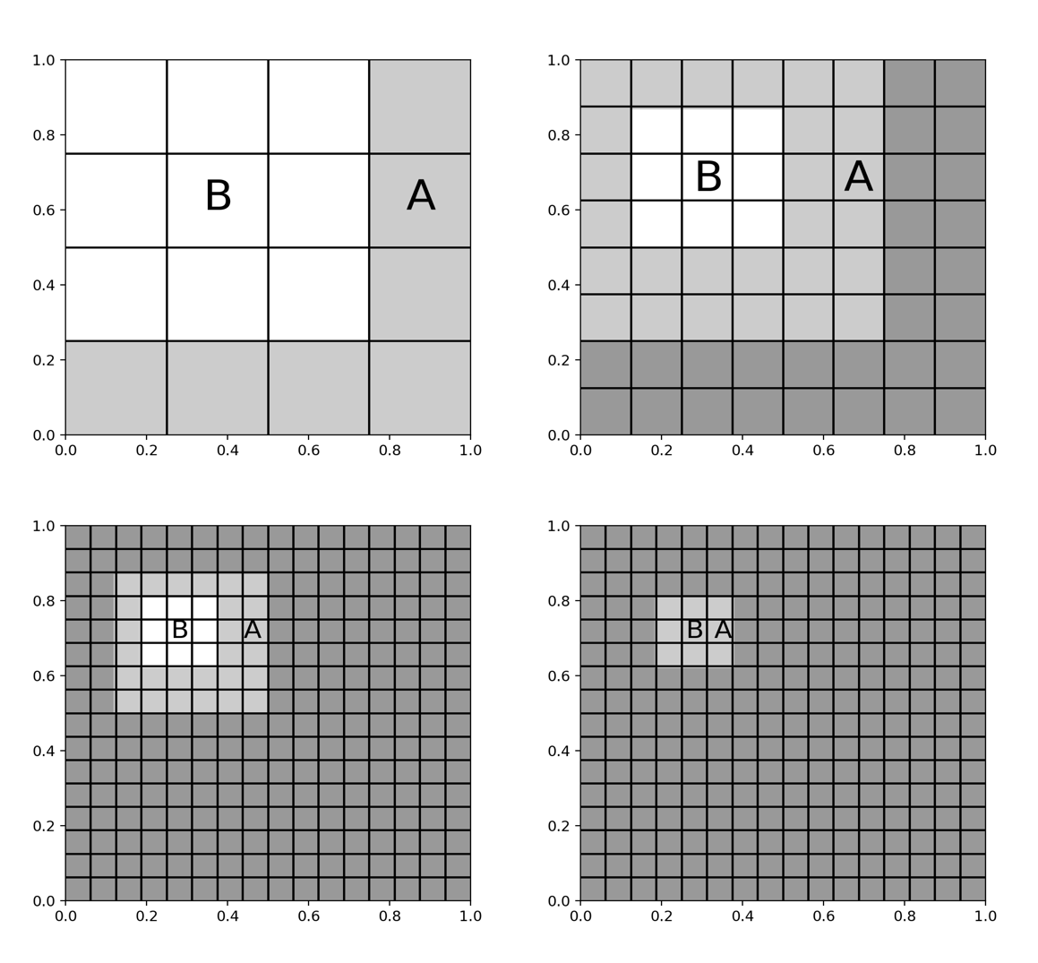 E. Read left to right, top to bottom. Light grey boxes are target boxes, being
evaluated for the source $B$. Dark grey boxes have been computed in the previous
recursive step.
E. Read left to right, top to bottom. Light grey boxes are target boxes, being
evaluated for the source $B$. Dark grey boxes have been computed in the previous
recursive step.
Now, if we can also reduce the number of steps, then we will observe the promised improvement in complexity, compared to direct computation.
In this analysis, I’ve ignored things like accuracy, which will be pretty terrible as in general $A$ and $B$ have been only 1 box away from each other. In practice better approximations are available, but these will have to be saved for future posts. However I hope this has illustrated how some clever recursion can make such a massive improvement in a problem that on the face of it seems bounded by a very poor time complexity.
References
[1] L. Ying, “A pedestrian introduction to fast multipole methods,” Sci. China Math., vol. 55, no. 5, pp. 1043–1051, 2012.